Univariable analysis

1. Learning outcomes

At the end of the session, participants will be able to:

Perform hypothesis tests.
Estimate risk ratios (also called relative risk) for categorical data.
Interpret the univariable results.
(Optional) Investigate dose-response relationships in categorical data.

2. Story/plot description

You have just estimated risk ratios (RR) of individual food items manually to better understand the concept. RR give you an idea of which food items could be the culprit(s) of the outbreak.

Now, you will practice performing hypothesis testing and calculating RR in R to investigate the associations of suspicious food items with the disease.

Note that, although this is not an exhaustive list of tests, the following can be useful for this exercise (relevant for comparisons between two groups):

For continuous variables:
- shapiro.test() (for checking if normally distributed)
- t.test() (for normal distributions)
- wilcox.test() (for non-parametric testing. Used to determine if two numeric samples are from the same distribution, when their populations are not normally distributed or have unequal variance.)
For categorical variables:
- chisq.test() (if all comparisons include at least 5 cases)
- fisher.test() (if there are < 5 cases for any comparison)

3. Questions/Assignments

3.1. Install packages and load libraries

Show the code

# Load the required libraries into the current R session:
pacman::p_load(rio, 
               here, 
               tidyverse, 
               skimr,
               plyr,
               janitor,
               lubridate,
               gtsummary, 
               flextable,
               officer,
               epikit, 
               apyramid, 
               scales,
               EpiStats,
               broom)

3.2. Import your data

Show the code

# Import the raw data set:
copdata <- rio::import(here::here("data", "Spetses_clean2_2024.rds"), trust = T)

3.3. Hypothesis tests for other variables

Check if the following variables are associated with being a case: age, sex, class and group.

a) age

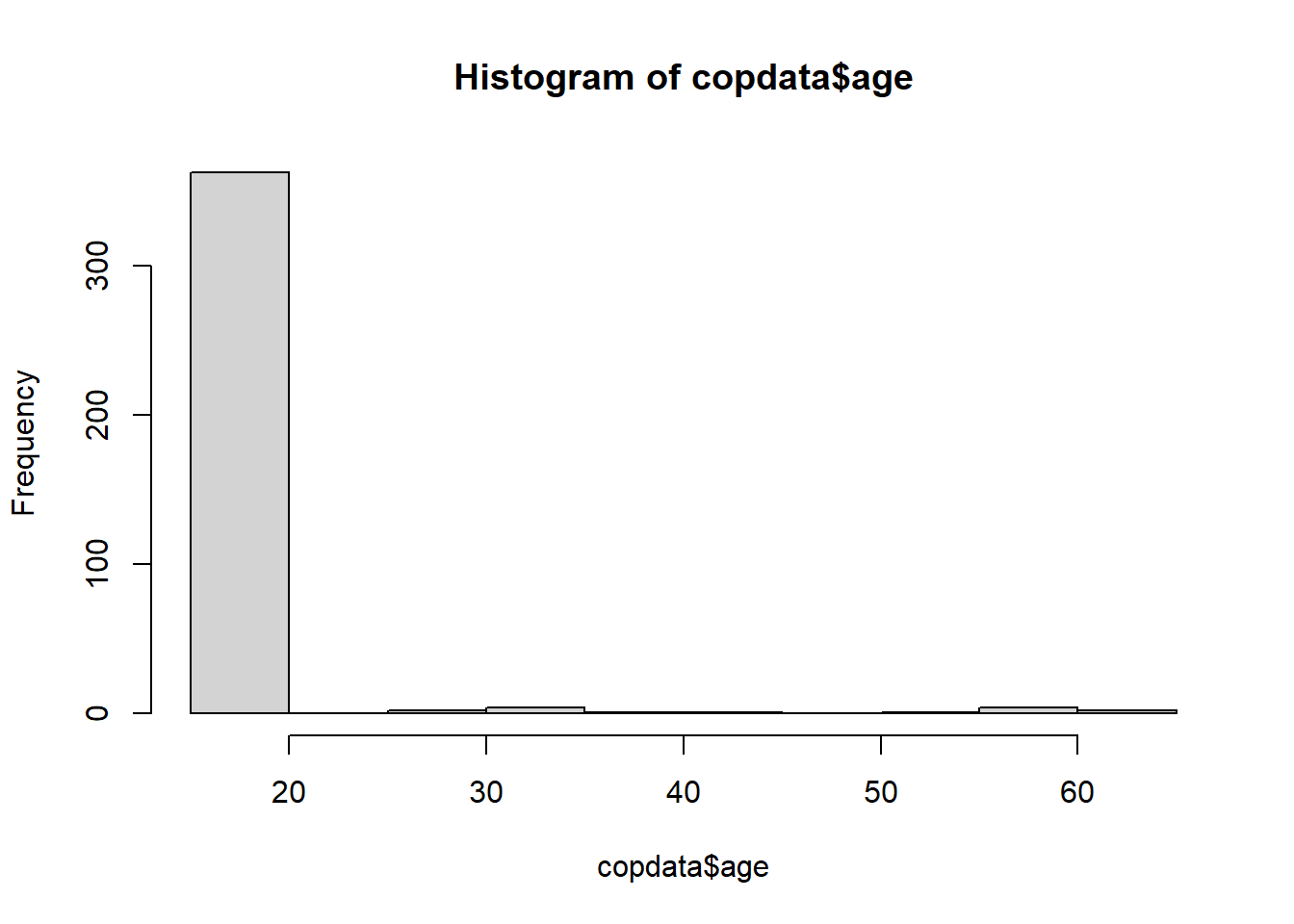
With the Shapiro-Wilk test we check if the variables are following the normal distribution. The null hypothesis is that the data follow a normal distribution, therefore, rejecting the null hypothesis means that the data do not follow the normal distribution. A p-value below the cutoff for rejecting the null hypothesis, e.g., a p-value<0.05 means that we reject the null hypothesis that the data follow the normal distribution. For age, the p-value is <0.05, therefore we reject the null hypothesis that the data are normally distributed. As we see in the graph most frequently reported age is <20 years.

Show the code

# Check if age overall follows a normal distribution:
shapiro.test(copdata$age)


    Shapiro-Wilk normality test

data:  copdata$age
W = 0.31302, p-value < 2.2e-16

Show the code

# Can simply have a look at
hist(copdata$age)

Show the code

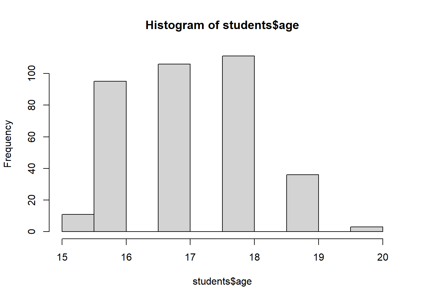
# Looking only at the students:
students <- copdata %>% 
  filter(group == "student")
hist(students$age)

Age overall (nor within the students’ group) is not normally distributed.

We compare the age for cases and non-cases using the Wilcoxon test that is used when the data are not normally distributed. The null hypothesis is that there is no difference in the age between the two groups compared. Given that p-value>0.05 we do not reject the null hypothesis.

Show the code

# Perform Wilcoxon rank sum test on age and sex:
wilcox.test(age ~ case, 
            data = copdata)


    Wilcoxon rank sum test with continuity correction

data:  age by case
W = 15934, p-value = 0.1512
alternative hypothesis: true location shift is not equal to 0

b) sex

Show the code

copdata %>% 
  select(sex, case) %>% 
  tbl_summary(by = case) %>% 
  add_p()

Characteristic	0 N = 161¹	1 N = 216¹	p-value²
sex			0.3
female	96 (60%)	117 (54%)
male	65 (40%)	99 (46%)
¹ n (%)
² Pearson’s Chi-squared test

Let’s stop and… think!

What do these results tell you - is there an association between sex and being a case?

Do these results differ from what you expected when looking at the descriptive figures (case proportions stratified by sex, or the age sex pyramid)? If so, why do you think this is?

c) class

Show the code

copdata %>% 
  select(class, case) %>% 
  tbl_summary(by = case) %>% 
  add_p()

Characteristic	0 N = 161¹	1 N = 216¹	p-value²
class			0.090
1	63 (43%)	68 (34%)
2	44 (30%)	57 (29%)
3	38 (26%)	73 (37%)
Unknown	16	18
¹ n (%)
² Pearson’s Chi-squared test

In this case you have a 2x3 contingency table of class against disease status, we can use a chi-square here. P-value of the association between class and age is p-val = 0.09, suggesting that there is an association at the p-val = 0.20 level among at least one of the 3 different classes. Fellows may want to investigate this further, but in the remaining of the study this is not explored further.

A hypothesis could be that one of the classes sat together and, for whatever reason, they ate more of the contaminated food item at those tables. This could be further studied if we had the spatial distribution of where the people sat at the dinner. Another hypothesis is that one of the classes differ from other classes in some characteristics that made them more susceptible or more exposed to the infected food item.

d) group

Show the code

copdata %>% 
  select(group, case) %>% 
  tbl_summary(by = case) %>% 
  add_p()

Characteristic	0 N = 161¹	1 N = 216¹	p-value²
group			0.2
teacher	9 (5.6%)	6 (2.8%)
student	152 (94%)	210 (97%)
¹ n (%)
² Pearson’s Chi-squared test

P-value of the association between group and age is p-val = 0.2, suggesting that there may be an association at the p-val = 0.20 level. Explanations are like above, with variable class.

Let’s do all together

Show the code

copdata %>% 
  select(sex, class, group, case) %>% 
  tbl_summary(by = case) %>% 
  add_p()

Characteristic	0 N = 161¹	1 N = 216¹	p-value²
sex			0.3
female	96 (60%)	117 (54%)
male	65 (40%)	99 (46%)
class			0.090
1	63 (43%)	68 (34%)
2	44 (30%)	57 (29%)
3	38 (26%)	73 (37%)
Unknown	16	18
group			0.2
teacher	9 (5.6%)	6 (2.8%)
student	152 (94%)	210 (97%)
¹ n (%)
² Pearson’s Chi-squared test

3.4. Risk Ratios

The risk ratios of each food item (including the 2x2 table) are reported below. The output of the CS() command is two tables: one with the 2x2 table and one with the risk difference, the risk ratio and the attributable fraction among exposed as well as the attributable fraction among the population (and the confidence intervals for all the estimates). The Chi-square and the p-value are also reported. In the second part, a table with all the food items is printed including attack rates for exposed and unexposed as well as risk ratios and the 95% confidence intervals (CI ll and CI ul, for the lower and upper interval) and p-values.

a) Calculate 95% CI Risk Ratios for food

To see if food items (note these are categorical variables) are associated with being a case, calculate risk ratios and 95% confidence intervals for food items. You can calculate this individually for each food item (using CSTable()), or all at once (see hint below).

Need a little bit of help?

Create a food_vars vector containing food variables of interest and use the function CSTable() of the EpiStats package.

Using this hint, you will create a table with the name of exposure variables, the total number of exposed, the number of exposed cases, the attack rate among the exposed, the total number of unexposed, the number of unexposed cases, the attack rate among the unexposed, risk ratios, 95% percent confidence intervals, and p-values. Amazing, isn’t it? Have a look at ??CSTable to learn more.

Show the code

# You could use the EpiStats package for each food item
CS(copdata, "case", "feta")

$df1
          Cases Non Cases Total Risk
Exposed     156       115   271 0.58
Unexposed    60        42   102 0.59
Total       216       157   373 0.58

$df2
                Point estimate 95%CI.ll 95%CI.ul
Risk difference          -0.01    -0.12     0.10
Risk ratio                0.98     0.81     1.19
Prev. frac. ex.           0.02    -0.19     0.19
Prev. frac. pop           0.02       NA       NA
chi2(1)                   0.05       NA       NA
Pr>chi2                  0.826       NA       NA

Show the code

CS(copdata, "case", "sardines")

$df1
          Cases Non Cases Total Risk
Exposed     150       105   255 0.59
Unexposed    65        52   117 0.56
Total       215       157   372 0.58

$df2
                Point estimate 95%CI.ll 95%CI.ul
Risk difference           0.03    -0.08     0.14
Risk ratio                1.06     0.87     1.28
Attr. frac. ex.           0.06    -0.14     0.22
Attr. frac. pop           0.04       NA       NA
chi2(1)                   0.35       NA       NA
Pr>chi2                  0.553       NA       NA

Show the code

CS(copdata, "case", "eggplant")

$df1
          Cases Non Cases Total Risk
Exposed     123        93   216 0.57
Unexposed    83        60   143 0.58
Total       206       153   359 0.57

$df2
                Point estimate 95%CI.ll 95%CI.ul
Risk difference          -0.01    -0.12     0.09
Risk ratio                0.98     0.82     1.18
Prev. frac. ex.           0.02    -0.18     0.18
Prev. frac. pop           0.01       NA       NA
chi2(1)                   0.04       NA       NA
Pr>chi2                  0.837       NA       NA

Show the code

CS(copdata, "case", "pasta")

$df1
          Cases Non Cases Total Risk
Exposed     202       136   338 0.60
Unexposed    13        23    36 0.36
Total       215       159   374 0.57

$df2
                Point estimate 95%CI.ll 95%CI.ul
Risk difference           0.24     0.07     0.40
Risk ratio                1.65     1.06     2.58
Attr. frac. ex.           0.40     0.06     0.61
Attr. frac. pop           0.37       NA       NA
chi2(1)                   7.45       NA       NA
Pr>chi2                  0.006       NA       NA

Show the code

# You can save time (and probably typos!) by creating a vector for food variables...
food_vars <- c("feta", "sardines", "eggplant", "pasta", 
               "veal", "tomsal", "dessert", "bread",  
               "champagne", "beer", "redwine", "whitewine")

# ...and using EpiStats::CSTable() to run all variables together!
CSTable(copdata, "case", food_vars)

$df
          Tot.Exp Cases.Exp AR.Exp% Tot.Unexp Cases.Unexp AR.Unexp%   RR CI.ll
pasta         338       202   59.76        36          13     36.11 1.65  1.06
veal          338       201   59.47        36          14     38.89 1.53  1.01
champagne     316       187   59.18        48          21     43.75 1.35  0.97
tomsal        211       114   54.03       154          95     61.69 0.88  0.73
dessert       149        90   60.40       198         106     53.54 1.13  0.94
beer          281       166   59.07        78          41     52.56 1.12  0.89
redwine        80        42   52.50       259         150     57.92 0.91  0.72
sardines      255       150   58.82       117          65     55.56 1.06  0.87
whitewine     260       150   57.69        98          54     55.10 1.05  0.85
bread         342       196   57.31        29          16     55.17 1.04  0.74
feta          271       156   57.56       102          60     58.82 0.98  0.81
eggplant      216       123   56.94       143          83     58.04 0.98  0.82
          CI.ul p(Chi2)
pasta      2.58   0.006
veal       2.32   0.018
champagne  1.89   0.044
tomsal     1.04   0.144
dessert    1.36   0.202
beer       1.42   0.303
redwine    1.14   0.393
sardines   1.28   0.553
whitewine  1.29   0.659
bread      1.46   0.823
feta       1.19   0.826
eggplant   1.18   0.837

b) Prepare the RR table for publication

Need a little bit of help?

Use flextable() and set_header_labels().

Show the code

rr_tbl <- CSTable(copdata, "case", food_vars) %>% 
  as.data.frame() %>% 
  rownames_to_column() %>% 
  flextable() %>% 
   set_header_labels(
     values = c("Food Item",
                "Total exposed",     
               "Cases exposed", 
               "AR among exposed",    
               "Total unexposed",
               "Cases unexposed",
               "AR among unexposed",
               "RR",         
               "95% lower CI",             
               "95% upper CI",
               "p-value"))

Let’s stop and… think!

· What can you infer from this table?

· Considering the relative risks, which food or drink items do you think were most likely to be the vehicle(s) of infection in this outbreak?

· Do you think there are any confounders or effect modifiers? If so, how would you investigate these further?

The interesting results here are that the food items that are most suspicious are pasta,veal and champagne. Pasta as such is unlikely to be contaminated, but as you can see in the picture (and from the dinner night), it was served with pesto! Maybe it was the pesto? Who-ho-ho!

Before one jumps into conclusions, consider that this result could be due to confounding! Maybe pasta was “clean” but eaten by all the people who ate the food item that actually was contaminated!(Optional)

3.5. (Optional) Dose Response

Check for a dose-response relationship between the food items with the highest RR values (the top 3) and being a case.

a) Pasta

Using epitools::riskratio function:

Show the code

epitools::riskratio(copdata$pastaD,                     
                    copdata$case,                     
                    conf.level = 0.95)

$data
         Outcome
Predictor   0   1 Total
    0      23  13    36
    1      32  38    70
    2      76 107   183
    3      28  57    85
    Total 159 215   374

$measure
         risk ratio with 95% C.I.
Predictor estimate     lower    upper
        0 1.000000        NA       NA
        1 1.503297 0.9257878 2.441057
        2 1.619168 1.0310538 2.542742
        3 1.857014 1.1730804 2.939696

$p.value
         two-sided
Predictor  midp.exact fisher.exact chi.square
        0          NA           NA         NA
        1 0.081364161  0.100893180 0.07613202
        2 0.015337953  0.017069765 0.01373981
        3 0.002010616  0.002370887 0.00162311

$correction
[1] FALSE

attr(,"method")
[1] "Unconditional MLE & normal approximation (Wald) CI"

Using a binomial regression:

Show the code

# Let's get the results directly exponentiated
binom_pastaD_exp <- glm(case ~ pastaD, data = copdata, 
                       family = binomial(link = "log")) %>% 
  tidy(exponentiate = TRUE, 
       conf.int = TRUE)

binom_pastaD_exp

Let’s stop and… think!

What do these results tell you?

Results suggest a dose response relationship of having eaten pasta, pointing towards pasta as the potential vehicle. The higher the amount of pasta they ate, the stronger is the association (RR) with getting ill/being a case.

b) Veal

Using epitools::riskratio function:

Show the code

epitools::riskratio(copdata$vealD,
                    copdata$case,
                    conf.level = 0.95)

$data
         Outcome
Predictor   0   1 Total
    0      19  15    34
    1      30  40    70
    2      78 106   184
    3      33  54    87
    Total 160 215   375

$measure
         risk ratio with 95% C.I.
Predictor estimate     lower    upper
        0 1.000000        NA       NA
        1 1.295238 0.8431805 1.989659
        2 1.305797 0.8769752 1.944304
        3 1.406897 0.9314233 2.125090

$p.value
         two-sided
Predictor midp.exact fisher.exact chi.square
        0         NA           NA         NA
        1 0.22186384    0.2951163 0.21193013
        2 0.15357032    0.1884220 0.14587265
        3 0.07956697    0.1017336 0.07298506

$correction
[1] FALSE

attr(,"method")
[1] "Unconditional MLE & normal approximation (Wald) CI"

Using a binomial regression:

Show the code

# Binomial regression for RRs. 
# The outcome needs to be exponentiated so we can interpret it properly!
binom_vealD <- glm(case ~ vealD, data = copdata, 
             family = binomial(link = "log"))

# To get exponentiated:
binom_vealD_exp <- glm(case ~ vealD, data = copdata, 
                       family = binomial(link = "log")) %>% 
  tidy(exponentiate = TRUE, 
       conf.int = TRUE)

binom_vealD_exp

c) Champagne

Using epitools::riskratio function:

Show the code

epitools::riskratio(copdata$champagneD,                     
                    copdata$case,                     
                    conf.level = 0.95)

$data
         Outcome
Predictor   0   1 Total
    0      27  21    48
    1      93 111   204
    2      12  32    44
    3      24  44    68
    Total 156 208   364

$measure
         risk ratio with 95% C.I.
Predictor estimate     lower    upper
        0 1.000000        NA       NA
        1 1.243697 0.8812613 1.755193
        2 1.662338 1.1502014 2.402507
        3 1.478992 1.0260296 2.131923

$p.value
         two-sided
Predictor  midp.exact fisher.exact  chi.square
        0          NA           NA          NA
        1 0.188922591  0.201367850 0.183280359
        2 0.005584928  0.006247816 0.004961941
        3 0.027627736  0.036334120 0.025117641

$correction
[1] FALSE

attr(,"method")
[1] "Unconditional MLE & normal approximation (Wald) CI"

Using a binomial regression:

Show the code

# Let's get the results directly exponentiated
binom_champagneD_exp <- glm(case ~ champagneD, data = copdata, 
                       family = binomial(link = "log")) %>% 
  tidy(exponentiate = TRUE, 
       conf.int = TRUE)

binom_champagneD_exp

3.6 Summary

As a summary of what you’ve done above, answer these questions:

Is the respondents’ sex associated with being a case?
Is the school class associated with being a case?
Which foods increase the risk of being a case?
(Optional) Is there a dose-response relationship between the food items and being a case?
What do you think is the most likely culprit(s) of this outbreak at this point? Are there any risk factors you would like to highlight?